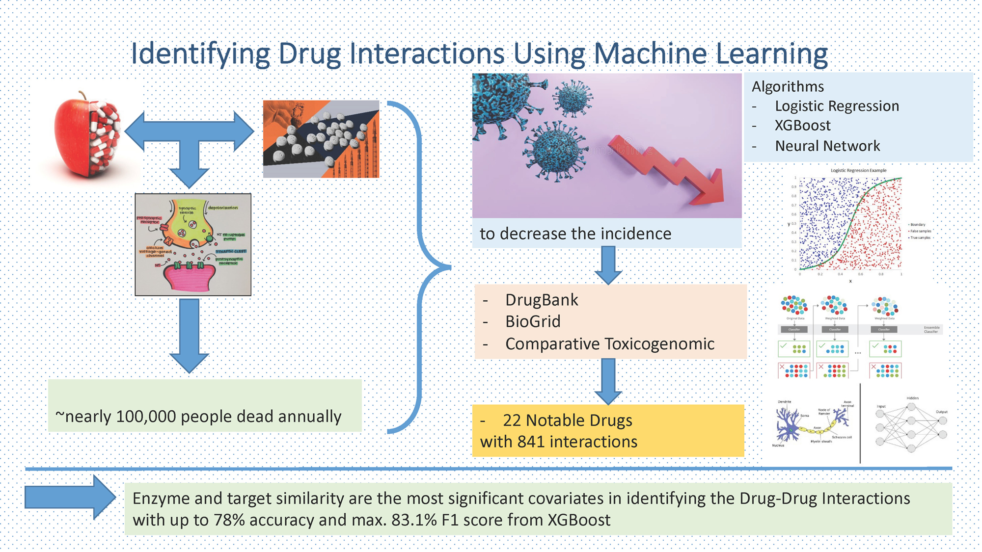
Abstract

The majority of Americans, accounting for 51% of the population, take 2 or more drugs daily. Unfortunately, nearly 100,000 people die annually as a result of adverse drug reactions (ADRs), making it the 4^th most common cause of mortality in the USA. Drug–drug interactions (DDIs) and their impact on patients represent critical challenges for the healthcare system. To reduce the incidence of ADRs, this study focuses on identifying DDIs using a machine-learning approach. Drug-related information was obtained from various free databases, including DrugBank, BioGRID and Comparative Toxicogenomics Database (CTD). Eight similarity matrices between drugs were created as covariates in the model in order to assess their influence on DDIs. Three distinct machine learning algorithms were considered, namely, logistic regression (LR), eXtreme Gradient Boosting (XGBoost) and neural network (NN). Our study examined 22 notable drugs and their interactions with 841 other drugs from DrugBank. The accuracy of the machine learning approaches ranged from 68% to 78%, while the F1 scores ranged from 78% to 83%. Our study indicates that enzyme and target similarity are the most significant parameters in identifying DDIs. Finally, our data-driven approach reveals that machine learning methods can accurately predict DDIs and provide additional insights in a timely and cost-effective manner.

Key words: prediction, machine learning algorithms, drug–drug interaction, similarity matrices, biostatistics

Introduction

A drug interaction occurs when one drug affects another drug by increasing or decreasing its effect. The manipulated effect of the drug might cause unwanted and unexpected side effects. Important pharmacological cycles that impact bioavailability, including assimilation, dissemination, digestion, and discharge, may be influenced by communication.¹ Such associations can incorporate issues like the organization of a medication that raises digestive system motility and decreases the retention of other medications, as well as the rivalry for a similar plasma protein carrier, restraint of the activity of an administered medication, or a communication at the discharge level, which influences the end of one of the medications.² Additionally, pharmacodynamic interactions may take place at the pharmacological level when 2 drugs interact with the same protein, at the signal level involving different signaling pathways, or at the effector level where different pharmacological responses are elicited.³ Hence, it is not feasible to identify or predict all drug interactions. However, it is possible to evaluate and comprehend the most important features affecting drug–drug interactions (DDIs) using the approach proposed in our study. Our method provides satisfactory results and insight into which covariates are most used while identifying DDIs.

Three types of approach are mainly implemented to predict DDI methods using machine learning approaches: 1) a similarity-based approach, 2) a classification-based approach and 3) a text mining approach. Some examples of these methods⁴ use similarity-based modeling with few similarity matrices such as 2D molecular structure, interaction profile, target, and side-effect similarities. On the other hand,⁵ some use a large-scale logistic regression (LR) model to predict potential DDIs. From the chemical–protein interactome (CPI) profile-based similarity to MeSH-based similarity, 10 similarities were used.⁶ Wu et al. provided a 3-tiered hierarchical text mining approach for Drug-Drug Interaction (DDI) analysis, designed to label essential terms, sentences containing drug interactions, and pairs of interacting drugs.⁶ However, text mining was not preferred by researchers, as they used classification-based approach⁷ to apply a new trend of similarity-based methods. Using the idea proposed by Vilar et al., a weighted similarity network was developed.² Similarly, Rohani and Eslahchi used a feature matrix with only using one machine learning algorithm, a neural network (NN).⁷ Most of these classification-based machine learning algorithms only use either a predictor or multiple predictors which are similar to other researches with LR. We offer to use more predictors with advanced machine learning algorithms.

Predicting DDIs can be investigated as a binary classification problem,^{7, 8} where the dependent variable is the interaction or non-interaction; the goal is to correctly label the DDIs. Our method uses feature matrices with classification-based machine learning algorithms, not only to compare different algorithms but also to write and create our dataset, as explained in Feature matrices section. In Materials and methods section, we pointed out where the data was collected and which databases were used. Additionally, we briefly introduced the machine learning algorithms used in the paper. Sample feature matrices are shown in Table 1. The first 2 columns stand for drug 1 and drug 2 names, others represent 8 feature matrices. Each of them, independently, shows how similar 2 drugs are based on a specific feature. Under the drug name, there is a code that stands for the DrugBank ID for that specific drug. It helps to work on drugs based on data structures such as split and merge. In Table 1, DB00176 stands for fluvoxamine which is a serotonin reuptake inhibitor used to treat obsessive-compulsive disorder. Fluvoxamine is also one of the most used antidepressants with cardiovascular drugs.⁹ Therefore, it has been chosen for illustration purposes in Table 1. The drugs in the 2^nd column were chosen randomly. For example, DB00717 stands for norethisterone, a progesterone used for birth control. The table can read Pathway similarities between them as 0.881, Medical Dictionary for Regula­tory Activities (MedDRA) (side effect) similarities as 0.171, ATC similarities as 0.000, enzyme similarities as 0.179, and so on. Feature matrices section explains the methods used to compute each column. In the Data analysis section, the methods of data analysis are described in detail. The data were fitted using 3 machine learning algorithms and the obtained minimum accuracy was 68.64%, the minimum F1 score was 78.16% from LR, the maximum accuracy was 78.12%, and the maximum F1 score was 83.1% from eXtreme Gradient Boosting (XGBoost) (Table 2). In Conclusions section, the importance of features is explained, and the most important covariate for explaining DDIs is plotted for trained data. Finally, future work is discussed.

Materials and methods

When a patient takes numerous medications, clinical DDIs can develop. Clinical toxicity or treatment failures can be caused by these DDIs. Therefore, DDI evaluations are an important element of medication development and the risk–benefit analysis of novel treatments. In their DDI guidance documents, regulatory agencies such as the Food and Drug Administration (FDA) of the USA, the Pharmaceuticals and Medical Devices Agency (PMDA) of Japan, and the European Medicines Agency (EMA) have recommended various methodologies (in vitro, clinical, and in silico) to examine DDI potentials, which can be utilized with patient management strategies. In this project, we conducted non-clinical DDI testing. Therefore, in this paper, publicly available databases were used. The following databases were used:

• DrugBank: A freely available database that stores drug information such as the Anatomical Therapeutic Chemical (ATC) codes enzymes, transporters and interactions;

• TwoSIDES: A freely available database with information about adverse drug reactions, side effects and drug indications;

• BioGRID: A public database that stores and disseminates data on genetic and protein interactions in human models and organisms;

• PubChem: A reference database for drug structures;

• UniProt: A database of protein sequences and functions that is open to the public.

Similarity metrics

Distance or similarity metrics were used in a broad range of applications, prompting evaluations of their effectiveness in fields such as texture image retrieval, web page clustering and social media event detection.¹⁰ The 3 most common similarity metrics include the Tanimoto coefficient, the Dice coefficient and the Cosine similarity.

The similarity values obtained using these methods were non-negative and included values between 0 to 1, including 0 and 1. When there was no similarity, a value of 0 was selected, and for many similarities, a value of 1 was chosen. The formulas compute these metrics and more can be found in Bajusz et. al.¹⁰ We mainly used Tanimoto similarity metrics while computing our feature matrices (Equation 1):

(1)

where a is the total number of objects in A, b is the total number of objects in B and c is the number of common objects between A and B, in which A and B stands for the features of drug 1 and drug 2.

Inverse document frequency

In the raw frequency, all terms are given equal importance.¹¹ However, it is known that some terms are repeated frequently, but they are not as important as once thought. Therefore, inverse document frequency (IDF) is a metric for determining whether a phrase is common or uncommon in a corpus of documents.¹² For example, after applying IDF for side effect (MedDRA) similarity, in the beginning, all of the reported side effects are counted, the number of unique side effects is identified, and a frequency table is created. Finally, the IDF of each unique side effect is computed using the following formula (Equation 2):

(2)

where N is the total number of documents, t denotes the interest, and df(t, drugs) denotes the number of medicines with the interest. If a side effect is reported frequently, it gets a smaller IDF number because of the natural logarithm of the fraction.

XGBoost

The XGBoost is one of the most preferred classification methods. It is not only computationally fast, but it also gives accurate results when compared to some other algorithms.¹³ The XGBoost is a tree-based algorithm that is similar to a decision tree; however, it uses a parallel computing feature. The XGBoost uses base/weak learners, which are only slightly better than guessing, but combines a bunch of the weak learners to create a strong learner, which is a form of ensemble learning. It weighs each weak learner prediction based on its prediction performance.¹⁴ The XGBoost uses 3 main forms of gradient boosting inside the algorithm. The learning rate is contained in gradient boosting, also known as the gradient boosting machine. For the training, test and validation sets, stochastic gradient boosting operates as a random sub-sample at the row and column level (if applicable). Finally, Regularized Gradient Boosting contains both L1, also known as Lasso regularization, and L2, also known as Ridge regularization. The XGBoost was chosen for this study because of its speed and excellent overall performance. The XGBoost constructs an ensemble of classification trees (as in classification and regression tree (CART)). When adding the t^th tree to the ensemble, the objective function for XGBoost can be formulated as follows (Equation 3):

(3)

where L(θ) denotes the loss function and Ω(θ) denotes the regulation function. More details of XGBoost can be found in Chen et al.¹⁵

Neural network

An NN is a computer program that uses algorithms to find patterns in a group of data.¹⁶ It resembles the work of human brain which tries to find relationships between things. In this context, a NN is a type of nervous system that can be biological or artificial.

A simple NN contains 3 layers: input, hidden and output. A layer is a collection of neurons. Usually, the number of hidden layers defines the name of the network. More details about NNs can be found in many valuable sources, such as the study by Paul and Singh.¹⁷ Activation functions are a very important part of NNs since they play a critical role in learning and understanding non-linear relationships between the input and output signals. The activation function in a NN receives a signal from the input, transforms it into an output signal, and sends it to the next layer. Except for the output layer, the rectified linear unit (ReLU) is a piecewise linear function used as an activation function because it has constraints on weights. When the value is less than 0, it takes 0; otherwise, it takes the obtained value.¹⁸ There are a few advantages of using ReLUs. Because of the constraint, taking the inverse of the function is easy. Moreover, ReLU does not activate all neurons, which helps in fast computation. For the output layer, sigmoid function has been chosen (Equation 4:

(4)

Sigmoid is mainly chosen because as an output we are interested in interaction (1) and non-interaction (0).¹⁹ In Equation 4, e stands for Euler’s number.

Logistic regression

Logistic regression is a statistical model in which dependent variables are categorical and have only 2 levels, such as success/failure and interaction/non-interaction. Principally, LR is suitable to test the hypothesis about relationships between a dichotomous response and one or more categorical or continuous explanatory variables.

Since LR can accommodate multiple-level categorical dependent variables, but we are interested in 2 levels only, we defined the basic LR form as follows (Equation 5):

(5)

where π is the probability of the outcome of interest, β₀ is the intercept, β₁ is the slope, and X is an arbitrary explanatory variable.

The LR-fitted line plot has a sigmoid or S-shaped curve and misrepresents data when using the linear regression line. Hence, LR uses logit, which stands for natural logarithm, to respond to variables. More details on LR can be found in the study by Peng et al.²⁰

Feature matrices

The DDI data were collected from different sources. DrugBank database v. 5.6. (https://go.drugbank.com; retrieved by June 2020) is a free drug information source that provides over 1.3 million accurate and updated DDIs covering all FDA- and Health Canada-approved drug sources from drug labels and references. Another free source, the Comparative Toxicogenomics Database (CTD) (http://ctdbase.org/downloads/; retrieved June 2020) is used for pathway and disease similarity. The TwoSIDES database (http://tatonettilab.org/resources/nsides/; retrieved June 2020) includes the information on adverse effects of the interacting drugs.

The DDI dataset, which was downloaded from DrugBank, was transformed into a matrix with dichotomous values [0,1] representing the interaction between 2 drugs. The extra columns take values between 0 and 1, which shows the similarity between the 2 drugs based on specific features such as chemicals, enzymes and proteins. When it comes to predicting new interactions, our method provides DDI predictions using the similarity between known DDIs and new drug pairs. Our basic assumption is that if drug A has a known interaction with drug B and the similarity between drug B and new drug C is greater than a certain threshold, then drug A will interact with drug C. If the 2 drugs are known to interact, and there is another drug that is comparable to one of the drugs in the DDI pair, the 3^rd drug can cause a DDI.

Feature vectors

One of the most important aspects of any statistical learning method is the extraction of a meaningful collection of features. Classic prediction studies primarily consider topological features. Ding et al. points that machine learning-based approaches can be divided into 3 groups.²¹ We combined all these types to create a feature matrix that contains approaches from all these types. In these types of setups, each feature matrix is an explanatory variable. Therefore, it would be beneficial to have as many feature matrices as possible. After an extensive literature review, we found out that creating the following feature matrices is feasible and advantageous.

Molecular structure similarity

To begin with, we present a specified collection of chemicals as simplified molecular-input line-entry system (SMILES) strings obtained from DrugBank. The RDKit was used to transform the SMILES strings into molecular extended connectivity fingerprints (ECFP; Open-Source Cheminformatics Software).²² The two-dimensional Tanimoto similarity measure, also known as the Jaccard similarity measure of the fingerprints, was used to calculate the similarity scores between 2 drug molecules.

ATC similarity

The World Health Organization (WHO) uses the Anatomical Therapeutic Chemical (ATC) classification system, which is a hierarchical classification system that organizes medications by organ or system. The ATC codes were gathered from DrugBank. Rednik’s semantic similarity algorithm was used to compute ATC similarity. This type of similarity was evaluated using ATC codes which are shown in Figure 1. The ATC coding system partitions are based on the biological system or organ on which they target.

Target similarity

Drug targets, such as specific proteins and nucleic acids, are a type of biological macromolecule in the body that has a pharmacodynamic function through interacting with medicines. To predict drug–target interactions (DTIs), several researchers used a single similarity measure for medications and targets, namely chemical structure similarity for pharmaceuticals and amino acid sequence similarity for targets. Amino acid sequences of the target proteins were obtained from the Universal Protein (UniProt) database. Then, the method suggested by Bleakley and Yamanishi²³ was used, namely the Smith–Waterman sequence alignment score between drug target genes computed with BLOSUM62 substitution matrix.²⁴ The scores’ geometric means were computed to normalize the score, which was obtained after aligning each sequence (Figure 2).

Pathway similarity

A drug’s target proteins are found in a variety of pathways, which means that a single drug can affect numerous pathways and modify their activities. Pathway information on drugs was obtained from the CTD.

We combined this information with DrugBank data. The IDF was used to assign more weight, and the Tanimoto coefficient was utilized to compute pathway similarities between pairs of drugs.

Disease similarity

Identifying drug–disease associations is time-consuming and expensive. Information on diseases associated with drugs was extracted from the CTD, in which the diseases associated with drugs were used for representing drug molecules. Then, we combined disease information with the DrugBank database. Finally, IDF was used to assign more weight and Tanimoto similarity was used to compute disease similarity between a pair of drugs.

MedDRA similarity

The MedDRA defines medical terminology to enable sharing of regulatory information. The terminology is used throughout the regulatory process, from pre-market to post-market, as well as for data entry, consultation, evaluation, and presentation. In the feature matrix, MedDRA is used for side-effect similarities. The side-effect information is gathered from TwoSIDES, which is a source of polypharmacy ADRs for combinations of drugs gathered from FDA Adverse Event Reporting System (FAERS) and the DrugBank. We have used IDF weight for the terms and computed Tanimoto coefficient for similarities between pairs of drugs.

Enzyme similarity

Enzyme similarity was computed using the approach applied to target similarity. Amino acid sequences of the enzyme protein were obtained using the UniProt database, and the Smith–Waterman sequence alignment score between drug target genes was computed as suggested by Bleakley and Yamanishi.²³ The geometric mean of the scores was calculated to normalize the score obtained from aligning each sequence.

PPI similarity

Proteins are in charge of all biological systems in a cell, and while many proteins operate on their own, the great majority of them interact with one another to ensure appropriate biological activity. The protein–protein interaction (PPI) network was created, and the closest distance between proteins was computed. Following the suggestions of Rohani and Eslahchi,⁷ the distances were converted to similarity measurements using the following equation (Equation 6):

(6)

where S(p₁,p₂) is the computed similarity value between 2 proteins, D(p₁,p₂) is the shortest path between these proteins in the PPI network, and A was chosen to be 0.9×exp(1). Figure 3 presents one-step interactions between proteins for illustration purposes.

Data analysis

This paper was intended to investigate major cardiovascular drugs and their interactions with other drugs. First, we took few well known drugs and their interaction to other available drugs. Then we added new drug and its interactions with other available. Finally, in the current study, we used 22 drugs in drug 1 column. In the current study, we used 22 drugs as drug 1 and 841 drugs as drug 2, totaling 18,249 data points after removing duplicates. Sample data is shown in Table 1. During the analysis, we used R v. 4.0.2 software (R Foundation for Statistical Computing, Vienna, Austria).

Checking for multicollinearity is a vital step of data analysis. Multicollinearity indicates which independent variables are not independent of each other, and whether the high correlation between independent variables might cause problems with not only fitting but also interpreting the results. Therefore, in Figure 4, the correlation matrix between 8 feature matrices can be observed. The highest correlation is 0.44 between Pathway similarity and Disease similarity. This is followed by a correlation 0.38 between Enzyme similarity and PPI similarity.

We checked the assumptions using LR and found that there were no highly influential outliers in the data. Cook’s distance was estimated to verify the finding. Linear relationships between each explanatory variable and the logit of the response variables were checked using the Box–Tidwell method. We have fitted a LR model, which contains both x and x*log(x) for all of our explanatory variables (x). We then added those interactions into a model and fitted it to LR. We found out that ATC, target, enzyme, and disease do not satisfy linearity assumptions. Their p-values were <2e-16, <2e-16, <2e-16, and 0.01747, respectively. Later, we created new variables using the square of ATC, target, enzyme, and disease. However, ATC was not significant. In the end, we used the square of the target, enzyme and disease variables, and the natural log of ATC. We checked all LR assumptions for new variables and did not notice any problems. Since we have a large dataset, overfitting was not our primary issue. The goodness-of-fit of the LR model was evaluated by using Nagelkerke’s R² from the fmsb R package and obtained a value of 0.2199, showing a moderate relationship. On the other hand, the model summary presented in Table 3 shows that all covariates are statistically significant.

Classification problems, especially with binary outcomes, were labeled as positive or negative. The decision was made by using a confusion matrix or contingency table, which consist of 4 categories: 1) true positive (TP) occurs when the outcome is successfully classified as positive; 2) true neg­ative (TN) occurs when the outcome is successfully clas­sified as negative; 3) false positive (FP) refers to an outcome as positive when the truth is negative; and 4) false negative (FN) refers to an outcome as negative when the truth is positive. Sensitivity refers to the ability of a test to correctly identify events related to a disease. Specificity, on the other hand, refers to the ability of a test to reliably detect events that occur in the absence of disease. Equation 7 has been used to compute these values in Table 2.

(7)

(8)

(9)

(10)

(11)

A confusion matrix can be obtained after fitting any machine learning algorithm and obtaining predictions on the test set. An accuracy of algorithm can be checked by computing some measures such as false positive rate (FPR) to indicate the fraction of negative groups which are incorrectly classified as positive. True positive rate (TPR) indicates the fraction of positive groups that are successfully classified as positive. Precision indicates the measure of correctly spotted positive events out of the predicted positive events. Recall indicates the measure of correctly spotted positive events out of all the actual positive events. Accuracy indicates the measure of all the correctly spotted events. When the ratio of the positive and negative events is close to each other, accuracy is a good indicator to consider. Although it is not always the case for equally numbered groups, in real datasets, mainly positive and negative events are not equal, which indicates imbalanced data. Therefore, an F1 score would be useful in the case of unequal groups and when FPs and FNs are being considered, since mislabeling interactions as non-interactions might cause patient’s death.

The dataset is split into branches (80% training and 20% testing). Three machine learning algorithms were used to fit the data in R software using the macOS Ventura 13.3.1 operating system (Apple Inc., Cupertino, USA). Results are shown in Table 2. We used the xgboost package to fit XGBoost, Keras and Tensorflow packages for fitting the NN and, finally, the stats package was used for fitting the LR. A 10-fold cross-validation was carried out independently for each algorithm to validate our models.

Conclusions

We have used 3 popular machine learning algorithms, LR, XGBoost and NN, for solving a classification problem. Each method has its strengths and weaknesses. Logistic regression is a simple algorithm that is easy to implement, interpret and explain. On the other hand, LR has limitations in its ability to capture complex, non-linear relationships between the dependent and independent variables. The XGBoost and NN are commonly preferred blackbox methods. They have high accuracy and power to handle larger datasets but time-consuming hyperparameter tuning and difficult interpretations.

Following the results presented in Table 2, we could say that using XGBoost would be a good machine learning algorithm in this case. We achieved the highest accuracy among all algorithms using XGBoost (78%), which is not surprising because, as we pointed out before, XGBoost uses gradient boosting inside the algorithm. Therefore, it is known to retrieve importance scores for each feature. In general, significance assigns a score to each feature that reflects how useful or important it was in the development of the model’s enhanced decision trees. The higher the relative relevance of a characteristic, the more often it is used to make critical judgments with decision trees. After the training, xgb.importance was used to identify which features have higher importance.²⁵ Feature selection is a widely used approach in machine learning.^{26, 27} Enzyme similarity is the most important feature in the model, followed by target similarity (Figure 5). Finally, ATC similarity is the least important feature. Thus, even if some papers are only focused on molecular similarity, enzyme and target protein similarities are the most vital features when it comes to identifying DDIs.

Kappa is a statistical measure that evaluates the degree of agreement between predicted and actual values. It ranges from −1 to 1, with 1 indicating perfect agreement, 0 indicating random agreement and −1 indicating complete disagreement. Based on the kappa values reported in Table 2, it is apparent that the XGBoost model exhibits the highest agreement between predicted and actual values, with a kappa value of 0.5508. This finding suggests that the XGBoost model is capable of predicting outcomes more accurately than the other 2 models. In contrast, the LR model reached the lowest kappa value of 0.2641. The NN model, with a kappa value of 0.4154, falls in between the values obtained for the XGBoost and LR models. These results suggest that the NN model is more accurate than the LR model but not as accurate as the XGBoost model in predicting outcomes.

Creating a new feature matrix is computationally requiring more powerful devices; therefore, using excessive feature matrices to identify DDIs in methods would would be interesting to investigate if the purpose is solely for feature selection in DDIs. However, we believe that after feature selection, the model would end up with 8 or 9 explanatory variables, which would be similar to the ones used in this paper. Additionally, we compared 3 machine learning algorithms, but every other classification method available in R programming could be used. Finally, we used 22 drugs as drug 1 and 841 drugs as drug 2 (see Table 1), but it could be expanded to larger numbers with more powerful devices and extra time, as mentioned earlier. Our method creates feature matrices from raw data and is still faster than many other approaches. The method would be vital for scientists in drug development since this is a non-clinical and accurate approach. It would also lower Research and Development (R&D) expenses of pharmaceutical companies. A R-shiny app or another automation system can be created to obtain probability of DDI interaction for chosen drugs. This would help doctors when deciding which drugs to prescribe for a given patient.

Supplementary data

The Supplementary file has 22 folders for each drugs in a drug 1 column in Table 1. The R codes which is used to fit all 3 machine learning algorithms can be found at https://github.com/iDemirsoy/Understanding-DDI-.